Get Started with Dgraph - Native Geolocation Features
Welcome to the eight tutorial of getting started with Dgraph.
In the previous tutorial, we learned about building a twitter-like user-search feature using Dgraph’s fuzzy search.
In this tutorial, we’ll build a graph of tourist locations around San Francisco and help our Zoologist friend, Mary, and her team in their mission to conserve birds using Dgraph’s geolocation capabilities.
You might have used Google to find the restaurants near you or to find the shopping centers within a mile of your current location. Applications like these make use of your geolocation data.
Geolocation has become an integral part of mobile applications, especially with the advent of smartphones in the last decade, the list of applications which revolves around users location to power application features has grown beyond imagination.
Let’s take Uber, for instance, the location data of the driver and passenger is pivotal for the functionality of the application. We’re gathering more GPS data than ever before, being able to store and query the location data efficiently can give you an edge over your competitors.
Real-world data is interconnected; they are not sparse; this is more relevant when it comes to location data. The natural representation of railway networks, maps, routes are graphs.
The good news is that Dgraph, the world’s most advanced graph database,
comes with functionalities to efficiently store and perform useful queries on graphs containing
location data. If you want to run queries like find me the hotels near Golden Gate Bridge,
or find me all the tourist location around Golden Gate Park, Dgraph has your back.
First, let’s learn how to represent Geolocation data in Dgraph.
Representing Geolocation data
You can represent location data in Dgraph using two ways:
- Point location
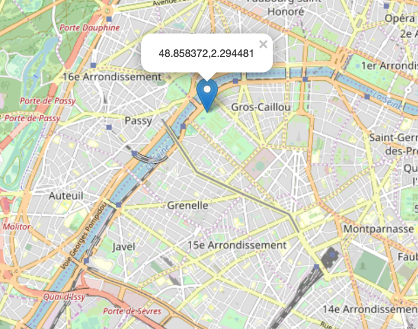
Point location contains the geo-coordinate tuple (latitude, longitude) of your location of interest.
The following image has the point location with the latitude and longitude for the Eifel tower in Paris. Point locations are useful for representing a precise location; for instance, your location when booking a cab or your delivery address.
- Polygonal location
It’s not possible to represent geographical entities which are spread across multiple geo-coordinates just using a point location. To represent geo entities like a city, a lake, or a national park, you should use a polygonal location.
Here is an example:
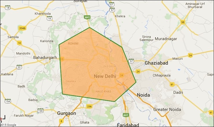
The polygonal fence above represents the city of Delhi, India. This polygonal fence
or the geo-fence is formed by connecting multiple straight-line boundaries, and
they are collectively represented using an array of location tuples of format
[(latitude, longitude), (latitude, longitude), ...]. Each tuple pair
(2 tuples and 4 coordinates) represents a straight line boundary of the geo-fence,
and a polygonal fence can contain any number of lines.
Let’s start with building a simple San Francisco tourist graph, here’s the graph model.
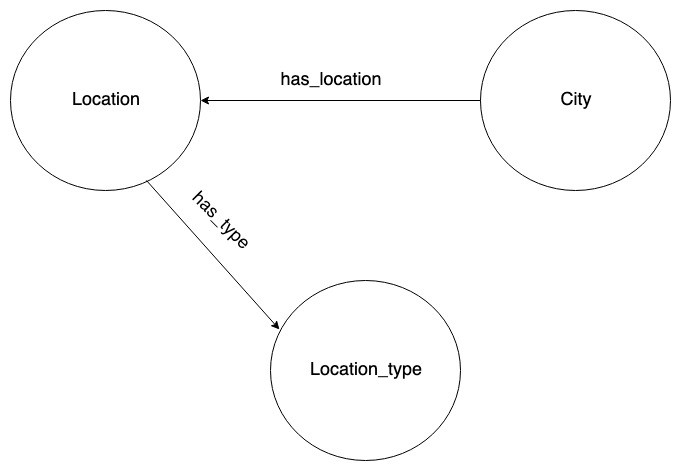
The above graph has three entities represented by the nodes:
- City
A city node represents the tourist city.
Our dataset only contains the city of San Francisco, and a node in the graph represents it.
- Location
A location node, along with the name of the location, it contains the point or polygonal location of the place of interest.
- Location Type
A location type consists of the type of location.
There are four types of location in our dataset: zoo, museum, hotel or a tourist attraction.
The location nodes with geo-coordinates of a hotel also contains their pricing information.
There are different ways to model the same graph.
For instance, the location type could just be a property or a predicate of the location node,
rather than being a node of its own.
The queries you want to perform or the relationships you like to explore mostly influence the modeling decisions. The goal of the tutorial is not to arrive at the ideal graph model, but to use a simple dataset to demonstrate the geolocation capabilities of Dgraph.
For the rest of the tutorial, let’s call the node representing a City as a city
node, and the node representing a Location as a location node, and the node
representing the Location Type as a location type node.
Here’s the relationship between these nodes:
- Every
city nodeis connected to alocation nodevia thehas_locationedge. - Every
location nodeis connected to its node representing alocation typevia thehas_typeedge.
Note: Dgraph allows you to associate one or more types for the nodes using its type system feature, for now, we are using nodes without types, we’ll learn about type system for nodes in a future tutorial. Check this page from the documentation site, if you want to explore type system feature for nodes.
Here is our sample dataset. Open Ratel, go to the mutate tab, paste the mutation, and click Run.
{
"set": [
{
"city": "San Francisco",
"uid": "_:SFO",
"has_location": [
{
"name": "USS Pampanito",
"location": {
"type": "Polygon",
"coordinates": [
[
[
-122.4160088,
37.8096674
],
[
-122.4161147,
37.8097628
],
[
-122.4162064,
37.8098357
],
[
-122.4163467,
37.8099312
],
[
-122.416527,
37.8100471
],
[
-122.4167504,
37.8101792
],
[
-122.4168272,
37.8102137
],
[
-122.4167719,
37.8101612
],
[
-122.4165683,
37.8100108
],
[
-122.4163888,
37.8098923
],
[
-122.4162492,
37.8097986
],
[
-122.4161469,
37.8097352
],
[
-122.4160088,
37.8096674
]
]
]
},
"has_type": [
{
"uid": "_:museum",
"loc_type": "Museum"
}
]
},
{
"name": "Alameda Naval Air Museum",
"location": {
"type": "Polygon",
"coordinates": [
[
[
-122.2995054,
37.7813924
],
[
-122.2988538,
37.7813582
],
[
-122.2988421,
37.7814972
],
[
-122.2994937,
37.7815314
],
[
-122.2995054,
37.7813924
]
]
]
},
"street": "Ferry Point Road",
"has_type": [
{
"uid": "_:museum"
}
]
},
{
"name": "Burlingame Museum of PEZ Memorabilia",
"location": {
"type": "Polygon",
"coordinates": [
[
[
-122.3441509,
37.5792003
],
[
-122.3438207,
37.5794257
],
[
-122.3438987,
37.5794587
],
[
-122.3442289,
37.5792333
],
[
-122.3441509,
37.5792003
]
]
]
},
"street": "California Drive",
"has_type": [
{
"uid": "_:museum"
}
]
},
{
"name": "Carriage Inn",
"location": {
"type": "Polygon",
"coordinates": [
[
[
-122.3441509,
37.5792003
],
[
-122.3438207,
37.5794257
],
[
-122.3438987,
37.5794587
],
[
-122.3442289,
37.5792333
],
[
-122.3441509,
37.5792003
]
]
]
},
"street": "7th street",
"price_per_night": 350.00,
"has_type": [
{
"uid": "_:hotel",
"loc_type": "Hotel"
}
]
},
{
"name": "Lombard Motor In",
"location": {
"type": "Polygon",
"coordinates": [
[
[
-122.4260484,
37.8009811
],
[
-122.4260137,
37.8007969
],
[
-122.4259083,
37.80081
],
[
-122.4258724,
37.8008144
],
[
-122.4257962,
37.8008239
],
[
-122.4256354,
37.8008438
],
[
-122.4256729,
37.8010277
],
[
-122.4260484,
37.8009811
]
]
]
},
"street": "Lombard Street",
"price_per_night": 400.00,
"has_type": [
{
"uid": "_:hotel"
}
]
},
{
"name": "Holiday Inn San Francisco Golden Gateway",
"location": {
"type": "Polygon",
"coordinates": [
[
[
-122.4214895,
37.7896108
],
[
-122.4215628,
37.7899798
],
[
-122.4215712,
37.790022
],
[
-122.4215987,
37.7901606
],
[
-122.4221004,
37.7900985
],
[
-122.4221044,
37.790098
],
[
-122.4219952,
37.7895481
],
[
-122.4218207,
37.78957
],
[
-122.4216158,
37.7895961
],
[
-122.4214895,
37.7896108
]
]
]
},
"street": "Van Ness Avenue",
"price_per_night": 250.00,
"has_type": [
{
"uid": "_:hotel"
}
]
},
{
"name": "Golden Gate Bridge",
"location": {
"type": "Polygon",
"coordinates": [
[
[
-122.479784,
37.8288329
],
[
-122.4775646,
37.8096291
],
[
-122.4775538,
37.8095165
],
[
-122.4775465,
37.8093304
],
[
-122.4775823,
37.8093296
],
[
-122.4775387,
37.8089749
],
[
-122.4773545,
37.8089887
],
[
-122.4773402,
37.8089575
],
[
-122.4772752,
37.8088285
],
[
-122.4772084,
37.8087099
],
[
-122.4771322,
37.8085903
],
[
-122.4770518,
37.8084793
],
[
-122.4769647,
37.8083687
],
[
-122.4766802,
37.8080091
],
[
-122.4766629,
37.8080195
],
[
-122.4765701,
37.8080751
],
[
-122.476475,
37.8081322
],
[
-122.4764106,
37.8081708
],
[
-122.476396,
37.8081795
],
[
-122.4764936,
37.8082814
],
[
-122.476591,
37.8083823
],
[
-122.4766888,
37.8084949
],
[
-122.47677,
37.808598
],
[
-122.4768444,
37.8087008
],
[
-122.4769144,
37.8088105
],
[
-122.4769763,
37.8089206
],
[
-122.4770373,
37.8090416
],
[
-122.477086,
37.809151
],
[
-122.4771219,
37.8092501
],
[
-122.4771529,
37.809347
],
[
-122.477179,
37.8094517
],
[
-122.4772003,
37.809556
],
[
-122.4772159,
37.8096583
],
[
-122.4794624,
37.8288561
],
[
-122.4794098,
37.82886
],
[
-122.4794817,
37.8294742
],
[
-122.4794505,
37.8294765
],
[
-122.4794585,
37.8295453
],
[
-122.4795423,
37.8295391
],
[
-122.4796312,
37.8302987
],
[
-122.4796495,
37.8304478
],
[
-122.4796698,
37.8306078
],
[
-122.4796903,
37.830746
],
[
-122.4797182,
37.8308784
],
[
-122.4797544,
37.83102
],
[
-122.479799,
37.8311522
],
[
-122.4798502,
37.8312845
],
[
-122.4799025,
37.8314139
],
[
-122.4799654,
37.8315458
],
[
-122.4800346,
37.8316718
],
[
-122.4801231,
37.8318137
],
[
-122.4802112,
37.8319368
],
[
-122.4803028,
37.8320547
],
[
-122.4804046,
37.8321657
],
[
-122.4805121,
37.8322792
],
[
-122.4805883,
37.8323459
],
[
-122.4805934,
37.8323502
],
[
-122.4807146,
37.8323294
],
[
-122.4808917,
37.832299
],
[
-122.4809526,
37.8322548
],
[
-122.4809672,
37.8322442
],
[
-122.4808396,
37.8321298
],
[
-122.4807166,
37.8320077
],
[
-122.4806215,
37.8319052
],
[
-122.4805254,
37.8317908
],
[
-122.4804447,
37.8316857
],
[
-122.4803548,
37.8315539
],
[
-122.4802858,
37.8314395
],
[
-122.4802227,
37.8313237
],
[
-122.4801667,
37.8312051
],
[
-122.4801133,
37.8310812
],
[
-122.4800723,
37.8309602
],
[
-122.4800376,
37.8308265
],
[
-122.4800087,
37.8307005
],
[
-122.4799884,
37.8305759
],
[
-122.4799682,
37.8304181
],
[
-122.4799501,
37.8302699
],
[
-122.4798628,
37.8295146
],
[
-122.4799157,
37.8295107
],
[
-122.4798451,
37.8289002
],
[
-122.4798369,
37.828829
],
[
-122.479784,
37.8288329
]
]
]
},
"street": "Golden Gate Bridge",
"has_type": [
{
"uid": "_:attraction",
"loc_type": "Tourist Attraction"
}
]
},
{
"name": "Carriage Inn",
"location": {
"type": "Polygon",
"coordinates": [
[
[
-122.3441509,
37.5792003
],
[
-122.3438207,
37.5794257
],
[
-122.3438987,
37.5794587
],
[
-122.3442289,
37.5792333
],
[
-122.3441509,
37.5792003
]
]
]
},
"street": "7th street",
"has_type": [
{
"uid": "_:attraction"
}
]
},
{
"name": "San Francisco Zoo",
"location": {
"type": "Polygon",
"coordinates": [
[
[
-122.5036126,
37.7308562
],
[
-122.5028991,
37.7305879
],
[
-122.5028274,
37.7305622
],
[
-122.5027812,
37.7305477
],
[
-122.5026992,
37.7305269
],
[
-122.5026211,
37.7305141
],
[
-122.5025342,
37.7305081
],
[
-122.5024478,
37.7305103
],
[
-122.5023667,
37.7305221
],
[
-122.5022769,
37.7305423
],
[
-122.5017546,
37.7307008
],
[
-122.5006917,
37.7311277
],
[
-122.4992484,
37.7317075
],
[
-122.4991414,
37.7317614
],
[
-122.4990379,
37.7318177
],
[
-122.4989369,
37.7318762
],
[
-122.4988408,
37.731938
],
[
-122.4987386,
37.7320142
],
[
-122.4986377,
37.732092
],
[
-122.4978359,
37.7328712
],
[
-122.4979122,
37.7333232
],
[
-122.4979485,
37.7333909
],
[
-122.4980162,
37.7334494
],
[
-122.4980945,
37.7334801
],
[
-122.4989553,
37.7337384
],
[
-122.4990551,
37.7337743
],
[
-122.4991479,
37.7338184
],
[
-122.4992482,
37.7338769
],
[
-122.4993518,
37.7339426
],
[
-122.4997605,
37.7342142
],
[
-122.4997578,
37.7343433
],
[
-122.5001258,
37.7345486
],
[
-122.5003425,
37.7346621
],
[
-122.5005576,
37.7347566
],
[
-122.5007622,
37.7348353
],
[
-122.500956,
37.7349063
],
[
-122.5011438,
37.7349706
],
[
-122.5011677,
37.7349215
],
[
-122.5013556,
37.7349785
],
[
-122.5013329,
37.7350294
],
[
-122.5015181,
37.7350801
],
[
-122.5017265,
37.7351269
],
[
-122.5019229,
37.735164
],
[
-122.5021252,
37.7351953
],
[
-122.5023116,
37.7352187
],
[
-122.50246,
37.7352327
],
[
-122.5026074,
37.7352433
],
[
-122.5027534,
37.7352501
],
[
-122.5029253,
37.7352536
],
[
-122.5029246,
37.735286
],
[
-122.5033453,
37.7352858
],
[
-122.5038376,
37.7352855
],
[
-122.5038374,
37.7352516
],
[
-122.5054006,
37.7352553
],
[
-122.5056182,
37.7352867
],
[
-122.5061792,
37.7352946
],
[
-122.5061848,
37.7352696
],
[
-122.5063093,
37.7352671
],
[
-122.5063297,
37.7352886
],
[
-122.5064719,
37.7352881
],
[
-122.5064722,
37.735256
],
[
-122.506505,
37.7352268
],
[
-122.5065452,
37.7352287
],
[
-122.5065508,
37.7351214
],
[
-122.5065135,
37.7350885
],
[
-122.5065011,
37.7351479
],
[
-122.5062471,
37.7351127
],
[
-122.5059669,
37.7349341
],
[
-122.5060092,
37.7348205
],
[
-122.5060405,
37.7347219
],
[
-122.5060611,
37.734624
],
[
-122.5060726,
37.7345101
],
[
-122.5060758,
37.73439
],
[
-122.5060658,
37.73427
],
[
-122.5065549,
37.7342676
],
[
-122.5067262,
37.7340364
],
[
-122.506795,
37.7340317
],
[
-122.5068355,
37.733827
],
[
-122.5068791,
37.7335407
],
[
-122.5068869,
37.7334106
],
[
-122.5068877,
37.733281
],
[
-122.5068713,
37.7329795
],
[
-122.5068598,
37.7328652
],
[
-122.506808,
37.7325954
],
[
-122.5067837,
37.732482
],
[
-122.5067561,
37.7323727
],
[
-122.5066387,
37.7319688
],
[
-122.5066273,
37.731939
],
[
-122.5066106,
37.7319109
],
[
-122.506581,
37.7318869
],
[
-122.5065404,
37.731872
],
[
-122.5064982,
37.7318679
],
[
-122.5064615,
37.731878
],
[
-122.5064297,
37.7318936
],
[
-122.5063553,
37.7317985
],
[
-122.5063872,
37.7317679
],
[
-122.5064106,
37.7317374
],
[
-122.5064136,
37.7317109
],
[
-122.5063998,
37.7316828
],
[
-122.5063753,
37.7316581
],
[
-122.5061296,
37.7314636
],
[
-122.5061417,
37.731453
],
[
-122.5060145,
37.7313791
],
[
-122.5057839,
37.7312678
],
[
-122.5054352,
37.7311479
],
[
-122.5043701,
37.7310447
],
[
-122.5042805,
37.7310343
],
[
-122.5041861,
37.7310189
],
[
-122.5041155,
37.7310037
],
[
-122.5036126,
37.7308562
]
]
]
},
"street": "San Francisco Zoo",
"has_type": [
{
"uid": "_:zoo",
"loc_type": "Zoo"
}
]
},
{
"name": "Flamingo Park",
"location": {
"type": "Polygon",
"coordinates": [
[
[
-122.5033039,
37.7334601
],
[
-122.5032811,
37.7334601
],
[
-122.503261,
37.7334601
],
[
-122.5032208,
37.7334495
],
[
-122.5031846,
37.7334357
],
[
-122.5031806,
37.7334718
],
[
-122.5031685,
37.7334962
],
[
-122.5031336,
37.7335078
],
[
-122.503128,
37.7335189
],
[
-122.5031222,
37.7335205
],
[
-122.5030954,
37.7335269
],
[
-122.5030692,
37.7335444
],
[
-122.5030699,
37.7335677
],
[
-122.5030813,
37.7335868
],
[
-122.5031034,
37.7335948
],
[
-122.5031511,
37.73359
],
[
-122.5031933,
37.7335916
],
[
-122.5032228,
37.7336022
],
[
-122.5032697,
37.7335937
],
[
-122.5033194,
37.7335874
],
[
-122.5033515,
37.7335693
],
[
-122.5033723,
37.7335518
],
[
-122.503369,
37.7335068
],
[
-122.5033603,
37.7334702
],
[
-122.5033462,
37.7334474
],
[
-122.5033073,
37.733449
],
[
-122.5033039,
37.7334601
]
]
]
},
"street": "San Francisco Zoo",
"has_type": [
{
"uid": "_:zoo"
}
]
},
{
"name": "Peace Lantern",
"location": {
"type": "Point",
"coordinates": [
-122.4705776,
37.7701084
]
},
"street": "Golden Gate Park",
"has_type": [
{
"uid": "_:attraction"
}
]
},
{
"name": "Buddha",
"location": {
"type": "Point",
"coordinates": [
-122.469942,
37.7703183
]
},
"street": "Golden Gate Park",
"has_type": [
{
"uid": "_:attraction"
}
]
},
{
"name": "Japanese Tea Garden",
"location": {
"type": "Polygon",
"coordinates": [
[
[
-122.4692131,
37.7705116
],
[
-122.4698998,
37.7710069
],
[
-122.4702431,
37.7710137
],
[
-122.4707248,
37.7708919
],
[
-122.4708911,
37.7701541
],
[
-122.4708428,
37.7700354
],
[
-122.4703492,
37.7695011
],
[
-122.4699255,
37.7693989
],
[
-122.4692131,
37.7705116
]
]
]
},
"street": "Golden Gate Park",
"has_type": [
{
"uid": "_:attraction"
}
]
}
]
}
]
}
Note: If this mutation syntax is new to you, refer to the first tutorial to learn the basics of mutations in Dgraph.
Run the query below to fetch the entire graph:
{
  entire_graph(func: has(city)) {
    city
    has_location {
    name
    has_type {
      loc_type
      }
    }
  }
}
Note: Check the second tutorial if you want to learn more about traversal queries like the above one.
Here’s our graph!
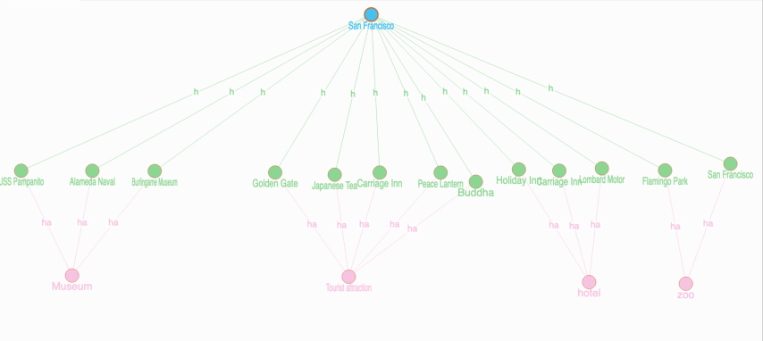
Our graph has:
- One blue
city node. We just have one node which represents the city ofSan Francisco. - The green ones are the the
locationnodes. We have a total of 13 locations. - The pink nodes represent the
location types. We have four kinds of locations in our dataset:museum,zoo,hotel, andtourist attractions.
You can also see that Dgraph has auto-detected the data types of the predicates from
the schema tab, and the location predicate has been auto-assigned geo type.
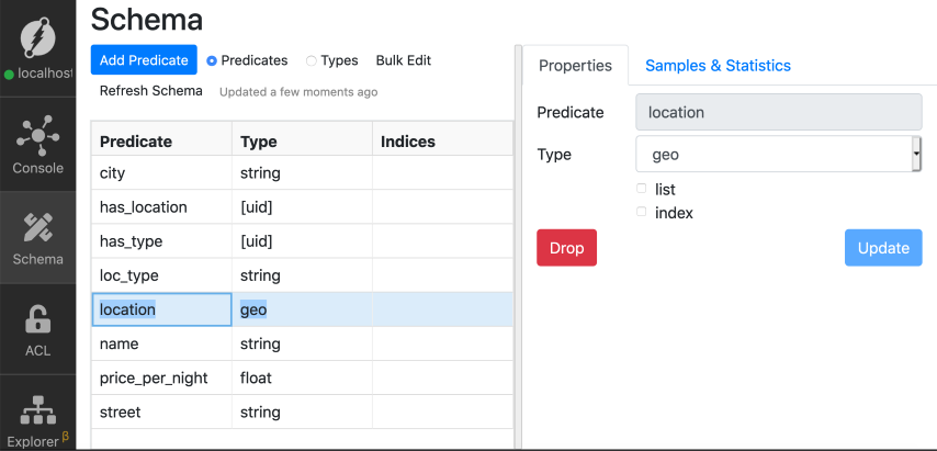
Note: Check out the previous tutorial to know more about data types in Dgraph.
Before we start, please say Hello to Mary, a zoologist who has dedicated her
research for the cause of conserving various bird species.
For the rest of the tutorial, let’s help Mary and her team of zoologists in their mission to conserving birds.
Enter San Francisco: Hotel booking
Several research projects done by Mary suggested that Flamingos thrive better when there are abundant water bodies for their habitat.
Her team got approval for expanding the water source for the Flamingos in the San Francisco Zoo, and her team is ready for a trip to San Francisco with Mary remotely monitoring the progress of the team.
Her teammates wish to stay close to the Golden Gate Bridge so that they could
cycle around the Golden gate, enjoy the breeze, and the sunrise every morning.
Let’s help them find a hotel which is within a reasonable distance from the
Golden Gate Bridge, and we’ll do so using Dgraph’s geolocation functions.
Dgraph provides a variety of functions to query geolocation data.
To use them, you have to set the geo index first.
Go to the Schema tab and set the index on the location predicate.
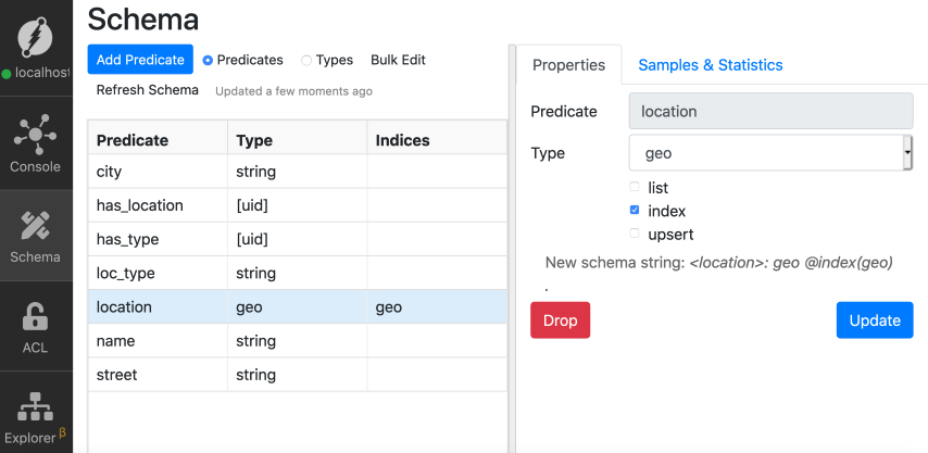
After setting the geo index on the location predicate, you can use Dgraph’s
built-in function near to find the hotels near the Golden gate bridge.
Here is the syntax of the near function: near(geo-predicate, [long, lat], distance).
The near function matches and
returns all the geo-predicates stored in the database which are within distance meters
of geojson coordinate [long, lat] provided by the user.
Let’s search for hotels within 7KM of from a point on the Golden Gate bridge.
Go to the query tab, paste the query below and click Run.
{
  find_hotel(func: near(location, [-122.479784,37.82883295],7000) )  {
    name
    has_type {
      loc_type
    }
  }
}
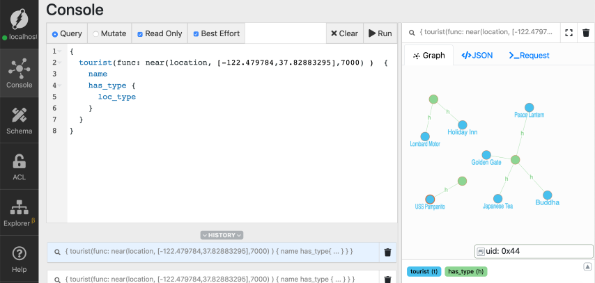
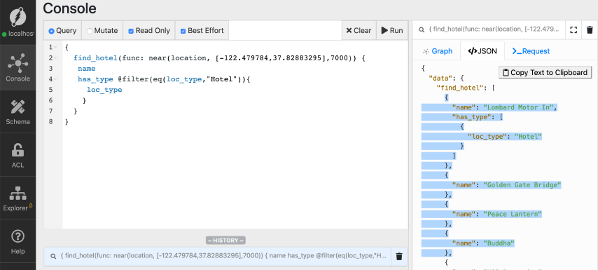
Wait! The search returns not just the hotels, but also all other locations
within 7 Km from the point coordinate on the Golden Gate Bridge.
Let’s use the @filter function to filter for search results containing only the hotels.
You can visit our third tutorial of the series
to refresh our previous discussions around using the @filter directive.
{
  find_hotel(func: near(location, [-122.479784,37.82883295],7000)) {
    name
    has_type @filter(eq(loc_type, "Hotel")){
      loc_type
    }
  }
}
Oops, we forgot to add an index while using the eq comparator in the filter.
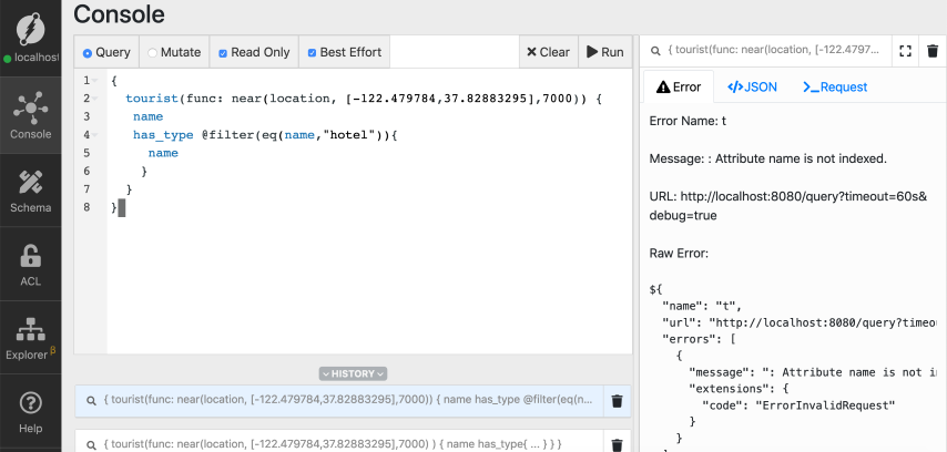
Let’s add a hash index to the loc_type and re-run the query.
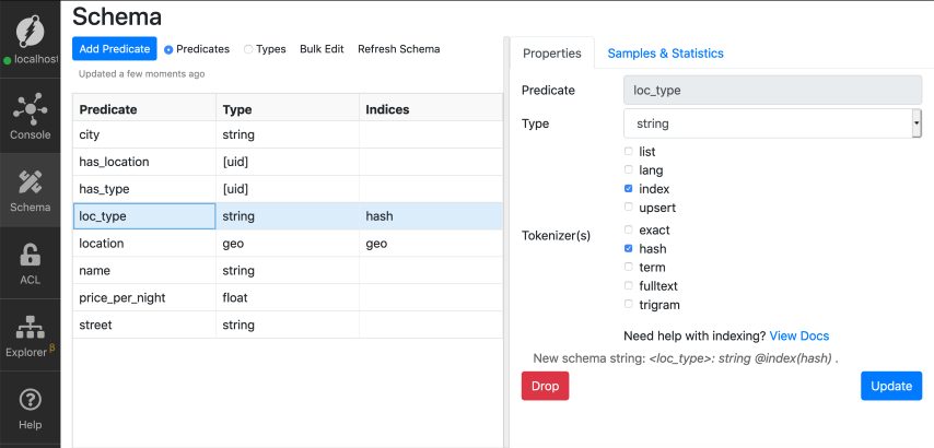
Note: Refer to the third tutorial of the series to learn more about hash index and comparator functions in Dgraph.
The search result still contains nodes representing locations which are not hotels.
That’s because the root query first finds all the location nodes which are within
7KM from the specified point location, and then it applies the filter while
selectively traversing to the location type nodes.
Only the predicates in the location nodes can be filtered at the root level, and
you cannot filter the location types without traversing to the location type nodes.
We have the filter to select only the hotels while we traverse the
location type nodes. Can we cascade or bubble up the filter to the
root level, so that, we only have hotels in the final result?
Yes you can! You can do by using the @cascade directive.
The @cascade directive helps you cascade or bubble up the filters
applied to your inner query traversals to the root level nodes, by doing
so, we get only the locations of hotels in our result.
{
  find_hotel(func: near(location, [-122.479784,37.82883295],7000)) @cascade {
   name
   price_per_night
   has_type @filter(eq(loc_type,"Hotel")){
     loc_type
    }
  }
}
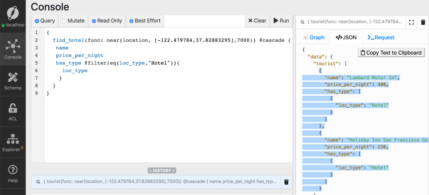
Voila! You can see in the result that, after adding the @cascade directive
in the query, only the locations with type hotel appear in the result.
We have two hotels in the result, and one of them is over their budget of 300$ per night. Let’s add another filter to search for Hotels priced below $300 per night.
The price information of every hotel is stored in the location nodes along with
their coordinates, hence the filter on the pricing should be at the root level of
the query, not at the level we traverse the location type nodes.
Before you jump onto run the query, don’t forget to add an index on the price_per_night predicate.
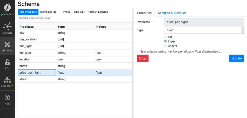
{
  find_hotel(func: near(location, [-122.479784,37.82883295],7000)) @cascade @filter(le(price_per_night, 300)){
    name
    price_per_night
    has_type @filter(eq(loc_type,"Hotel")){
      loc_type
    }
  }
}
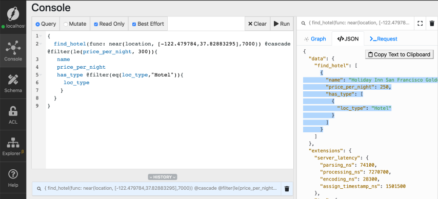
Now we have a hotel well within the budget, and also close to the Golden Gate Bridge!
Summary
In this tutorial, we learned about geolocation capabilities in Dgraph, and helped Mary’s team book a hotel near Golden bridge.
In the next tutorial, we’ll showcase more geolocation functionalities in Dgraph and assist Mary’s team in their quest for conserving Flamingo’s.
See you all in the next tutorial. Till then, happy Graphing!
Remember to click the “Join our community” button below and subscribe to our newsletter to get the latest tutorial right into your inbox.
What’s Next?
- Go to Clients to see how to communicate with Dgraph from your application.
- Take the Tour for a guided tour of how to write queries in Dgraph.
- A wider range of queries can also be found in the Query Language reference.
- See Deploy if you wish to run Dgraph in a cluster.
Need Help
- Please use discuss.dgraph.io for questions, feature requests, bugs, and discussions.